Volatility Depends On The Resolution

How realized volatility depends on sampling frequency

Friends,

Today we jump into another large learning post including a chart book and commentary.

In this document, you will:

• learn to compute realized volatility

• appreciate the difference between the sampling window and lookback

• learn to annualize realized volatility

• examine market data to see how realized volatility varies with the sampling period

[bong rip]

Let’s cook…

I was able to fit the whole post except the chartbooks in the body of this email but here’s the link to the full post. It’s better formatted and colored there. Again, the chartbook is too large for substack.

🔎Volatility Depends On The Resolution

Introduction

These short posts explain the relevant computations. If you have ever computed a standard deviation, you are 99% of the way there.

➕Computing Realized Volatility

It’s common to compute realized volatility or the standard deviation of returns.

• The formula commonly uses daily closing prices (ie daily returns). That’s the 1 in the formula. However, we can sample the volatility using longer windows. If you chose 5 instead of 1 you are “sampling the volatility weekly instead of daily”.

• N represents the lookback. The larger the N the larger the sample size.

• Since volatility is only sampled on business days:

  • a lookback that samples the vol weekly will have an N of about 52 in a year while a lookback that samples the vol daily will have 251 samples in a year

  • the longer your sampling period, the smaller the sample size for a given lookback

A word on μ in the realized volatility formula
It is not uncommon for traders to discard μ which is equivalent to setting it to zero. The easiest way to appreciate why is to imagine a stock whose logreturn is exactly 2% per day. The daily deviation from the mean logreturn of +2% would be 0, in turn, rendering the realized volatility measure zero! If a stock went up (or down) 2% per day and we concluded that volatility is zero, then it’s fair to say the measure is broken. By “de-trending” the formula by ignoring μ, you get a less biased measure. In practice, this matters less over shorter lookbacks where the “drift” is a smaller component of the volatility. If your lookback periods are long, the drift becomes significant. If the SP500 has an annual drift of +9% with a standard deviation is 16% the drift is a substantial portion of the volatility. The impact is an order of magnitude smaller for shorter lookbacks. On a daily basis the drift is 3 bps while the volatility is 100 bps.

🗓️Annualizing Realized Volatility

To be repetitive, take note of the two time periods involved:

1. The sampling window This can be daily, weekly, monthly, annual returns. It can even be a return based on tick vols (hourly, minutely…)

2. The lookback period This is how far back in time we are sampling returns

For example, we can sample:

• daily returns for the past month or year

• hourly returns for the past day or week

The lookback determined the sample size.

The sampling window determines our annualization factor.

💡Annualization factor examples

• daily = √251

• weekly = √52

• monthly = √12

• hourly = √(251 x 6.5) = √1631.5

*You can go crazy with this if you want. There are days when the markets close early, the number of periods varies with leap years or what day of the week January 1 falls on. But maintain a sense of proportion. Any error do to these differences will be swamped by the fact that all implied vols and realized vols are imperfect measures because time itself is linear while event or voltime is not. See ⏳Understanding Variance Time

You simply cannot exhaust how deep you can get into this. Where you draw the line depends on your strategy. 99.5% of strategies are robust to the approximations above.

Now we compute realized volatilities on actual historical prices to see what we can learn.

Data Exploration

Setup

Since we want to compare the effect of sampling period on realized volatility we will keep the lookback period constant.

As a reminder, if we computed daily volatility for the past 6 months:

• the sampling period is daily or 1 day

• the lookback is 6 months

We call this “6-month realized sampled daily”

Since volatility tends to “cluster” (low vol periods follow low vol periods and high vol periods tend to follow high vol periods), option markets for short or even medium terms maturities will give more weight to recent realized volatility. If you were pricing a 3-year option then you’d be more inclined to examine longer a longer lookback which smooths out the sharper peaks and valleys.

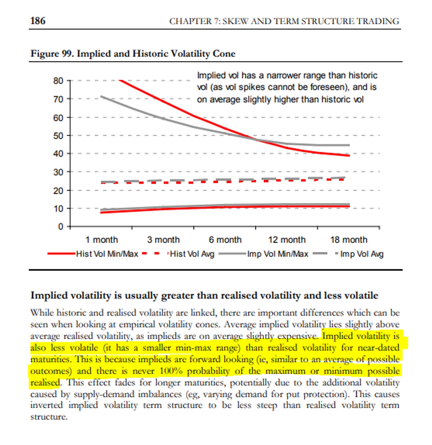
This idea is echoed in the concept of a “vol cone”

via Colin Bennett’s Volatility Trading

GLD Vol cone on 8/21/24 (courtesy of moontower.ai)

For our data exploration, we will

1. use constant lookback of 40 business days which is close to 2 months worth of trading days. We call this “40-day vol” .

2. sample the vol using daily, 2 day, 5d , 10d, and 20d windows.

   1. This maps to 40-day vol being computed from samples of the following quantities respectively:

      • daily (n = 40)

      • 2 day (n = 20)

      • 5d (n = 8)

      • 10d (n=4)

      • 20d (n =2)

3. compute 40-day vol for each business day from 1/2/2013 until 8/16/2024 (>11.5 years)

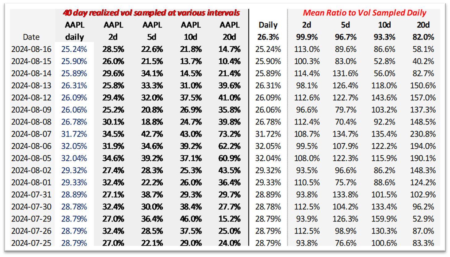
Example using AAPL

Let’s step through an example with AAPL.

1. We compute the realized vol for the 40 day lookback at with carious sampling windows.

   1. In the snippet below, we also compute the ratio vols from each sampling period to the realized vol computed from daily samples

      

2. Scatterplot the ratio of 40-day realized vol sampled at different frequencies vs 40-day realized vol sampled daily

   1. A point on the black dotted line means the 40-day vol sampled daily was the same as the 40-day vol at the respective frequency

   2. If a point is above the line, the vol sampled at a slower frequency is higher than the vol sampled daily (you might interpret this as a market that was trending. For example if a market went up 1% per day, then the daily vol would be about 16% but the 5d vol would be approximately 5% x √52 or 36%!

   3. The regressions show that vol sampled at slower frequencies is lower than vol sampled at a higher frequency.

      

3. Compute the aggregate stats for over 11.5 years There are 2 observations worth noting:

   1. The longer the sampling period, the lower the vol for the same 40-day lookback

      

   2. The standard deviation of that ratio grows with the sampling period. If sampling periods for the same lookback differ greatly there will be more variation in the measured realized vols relative to each other! The variation in the ratio by sampling period is easily seen with box-and-whisker charts

      

[See the main post for Chartbooks for various tickers]

Concluding thoughts

The most general results applied to every symbol:

• For a given lookback, less frequently sampled vol for a given lookback is biased lower. This echoes an earlier post Risk Depends on the Resolution

• However, in every case, the slower the sampling frequency (ie every 4 weeks instead of every 1 week), the more volatile the realized vol itself is compared to the daily sampled vol.

These results reinforce an intuitive idea: the longer your sampling period, the smaller the sample size for a given lookback, therefore:

The more frequently you sample vol the faster you converge on a better estimate of the volatility

If you only looked at annual returns it would take many years to get a sense of how volatile an asset or strategy is. This is also why evaluating investment managers on monthly returns is dangerous. It hides the risk.

Assorted observations:

• Periods when less frequently sampled vol give us a higher realized vol indicate trending (long option player will have wish they hedged less frequently or on a lower delta and vice versa!)

• Option traders think in straddles for shorter dated options but in vol for longer dated vols. Vol-thinking prompts you to ask “will this thing move X% per day” for the next year vs can this stock move 5% in a month. There’s a puzzle embedded in this revelation — the long gamma trader will conclude they should hedge daily to “capture” the higher vol, but a non-option trader may conclude that this is an argument for mean reversion on shorter time scales.

• An interesting scenario to filter for would a situation where realized volatility sampled slowly (ie weekly) was higher than higher frequency sampled vol for the same look back.

  • Like the earlier example of a stock that goes up 1% a day (16% realized vol sampled daily) vs >30% vol sampled weekly.

  • The reasoning here is: if the vol market is more focused on higher frequency sampled vol to price options it might underprice implied volatility.

  • I used the moontower.ai backend to filter for scenarios in a few names where monthly realized vol sampled every 3 days was higher than monthly realized vol sampled daily. I called the ratio “Trend Premium” so I filtered for situations where it was > 1.

    • I then filtered again where the options were cheap — a VRP < 1 (the RV in VRP coming from daily samples, making this analysis conservative)

This was an example from QQQ over the last 2 years.

The left chart highlights VRP < 1 AND “Trend premium” > 1

The right chart shows how the lagged VRP a month later (so what is the ratio of IV today divided by the realized vol that was eventually realized)

The realized vol underperformed the IV more than it usually does. So much for that. (I actually toggled through a bunch of names in this way but just eyeballing I couldn’t see a bias one way or the other. A sample of 2 years plus using overlapping data as it’s rolling windows is not exactly a proper study on this idea. The overlapping windows is not an issue for the general study earlier in the post which really just tries to understand the relationship of RV sampled at different frequencies for the same lookback. Overlapping windows does shrink your sample size if you are mining for a signal as I was flailing with this “Trend Premium” filter)

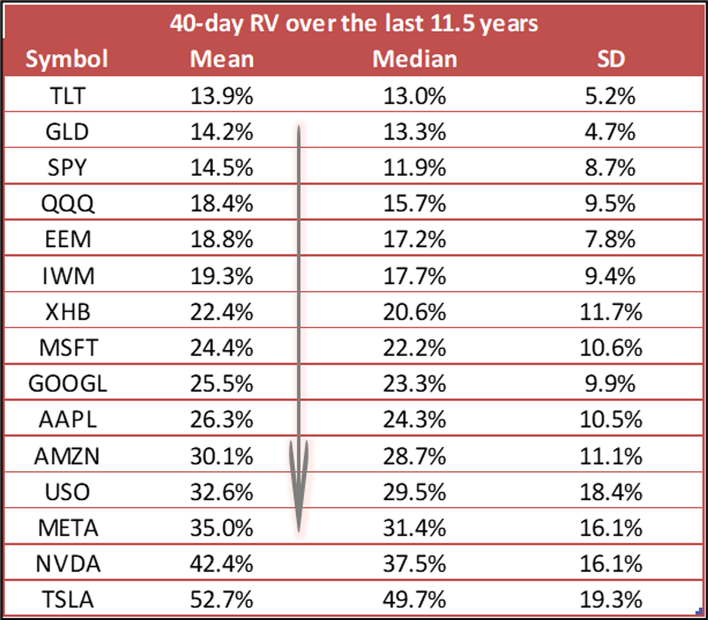
• Finally, here’s a summary table of the 40-day realized vol sampled daily for the past 11.5 years from our studies:

  

☮️

Stay groovy

---

If you got this far, you are a paying sub. It’s super appreciated and makes it easier to justify writing these long posts.

You can help moontower grow by referring even 1 person.

Use the affiliate link from this button and you accumulate credit towards comps:

Just copy and paste this to your friend:

Yo you should check this moontower substack out…it’s a total brain upgrade and most of the material is 100% free (although I pay because the paywalled stuff blue meth)

And there’s always these other upgrades if they suit: